Surrogate residuals

Simulate surrogate response values for cumulative link regression models using the latent method described in Liu and Zhang (2017).

resids(object, nsim = 1L, method = c("latent", "jitter"),
  jitter.scale = c("response", "probability"), ...)

Arguments

object	An object of class clm, glm, lrm, orm, polr, or vglm.
nsim	Integer specifying the number of bootstrap replicates to use. Default is 1L meaning no bootstrap samples.
method	Character string specifying which method to use to generate the surrogate response values. Current options are "latent" and "jitter". Default is "latent".
jitter.scale	Character string specifyint the scale on which to perform the jittering whenever method = "jitter". Current options are "response" and "probability". Default is "response".
...	Additional optional arguments. (Currently ignored.)

Value

A numeric vector of class c("numeric", "surrogate") containing the simulated surrogate response values. Additionally, if nsim > 1, then the result will contain the attributes:

boot_reps

A matrix with nsim columns, one for each bootstrap replicate of the surrogate values. Note, these are random and do not correspond to the original ordering of the data;

boot_id

A matrix with nsim columns. Each column contains the observation number each surrogate value corresponds to in boot_reps. (This is used for plotting purposes.)

Note

Surrogate response values require sampling from a continuous distribution; consequently, the result will be different with every call to surrogate. The internal functions used for sampling from truncated distributions are based on modified versions of rtrunc and qtrunc.

For "glm" objects, only the binomial() family is supported.

References

Liu, Dungang and Zhang, Heping. Residuals and Diagnostics for Ordinal Regression Models: A Surrogate Approach. Journal of the American Statistical Association (accepted). URL http://www.tandfonline.com/doi/abs/10.1080/01621459.2017.1292915?journalCode=uasa20

Nadarajah, Saralees and Kotz, Samuel. R Programs for Truncated Distributions. Journal of Statistical Software, Code Snippet, 16(2), 1-8, 2006. URL https://www.jstatsoft.org/v016/c02.

Examples

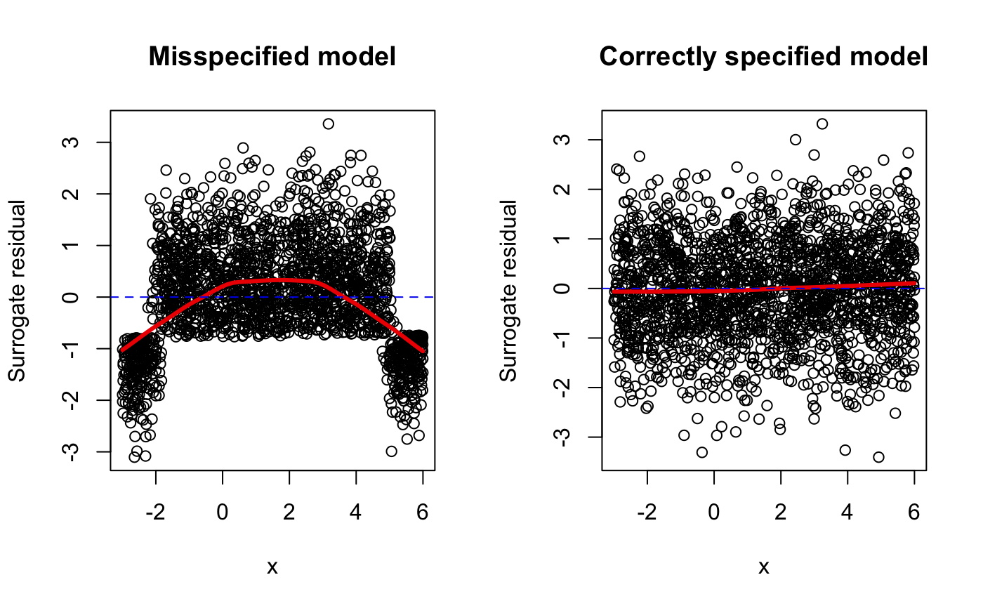
# Generate data from a quadratic probit model
set.seed(101)
n <- 2000
x <- runif(n, min = -3, max = 6)
z <- 10 + 3 * x - 1 * x^2 + rnorm(n)
y <- ifelse(z <= 0, yes = 0, no = 1)

# Scatterplot matrix
pairs(~ x + y + z)

# Setup for side-by-side plots
par(mfrow = c(1, 2))

# Misspecified mean structure
fm1 <- glm(y ~ x, family = binomial(link = "probit"))
scatter.smooth(x, y = resids(fm1),
               main = "Misspecified model",
               ylab = "Surrogate residual",
               lpars = list(lwd = 3, col = "red2"))
abline(h = 0, lty = 2, col = "blue2")

# Correctly specified mean structure
fm2 <- glm(y ~ x + I(x ^ 2), family = binomial(link = "probit"))
#> Warning: glm.fit: fitted probabilities numerically 0 or 1 occurred
scatter.smooth(x, y = resids(fm2),
               main = "Correctly specified model",
               ylab = "Surrogate residual",
               lpars = list(lwd = 3, col = "red2"))
abline(h = 0, lty = 2, col = "blue2")