Chapter 5 Deep Neural Networks (DNN)

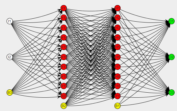
Image Source: https://machprinciple.wordpress.com/2013/11/09/neural-network-controlled-spacecraft-control-logic-exists/
5.1 Introduction
A Deep Neural Network (DNN) is an artificial neural network (ANN) with multiple hidden layers of units between the input and output layers. Similar to shallow ANNs, DNNs can model complex non-linear relationships. DNN architectures (e.g. for object detection and parsing) generate compositional models where the object is expressed as a layered composition of image primitives. The extra layers enable composition of features from lower layers, giving the potential of modeling complex data with fewer units than a similarly performing shallow network.
DNNs are typically designed as feedforward networks, but research has very successfully applied recurrent neural networks, especially LSTM, for applications such as language modeling. Convolutional deep neural networks (CNNs) are used in computer vision where their success is well- documented. CNNs also have been applied to acoustic modeling for automatic speech recognition, where they have shown success over previous models.
This tutorial will cover DNNs, however, we will introduce the concept of a “shallow” neural network as a starting point.
5.2 History
An interesting fact about neural networks is that the first artificial neural network was implemented in hardware, not software. In 1943, neurophysiologist Warren McCulloch and mathematician Walter Pitts wrote a paper on how neurons might work. In order to describe how neurons in the brain might work, they modeled a simple neural network using electrical circuits. [1]
5.3 Backpropagation
Backpropagation, an abbreviation for “backward propagation of errors”, is a common method of training artificial neural networks used in conjunction with an optimization method such as gradient descent. The method calculates the gradient of a loss function with respect to all the weights in the network. The gradient is fed to the optimization method which in turn uses it to update the weights, in an attempt to minimize the loss function.
5.4 Architectures
5.4.1 Multilayer Perceptron (MLP)
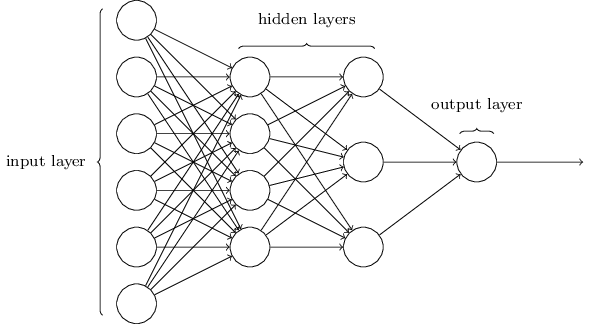
A multilayer perceptron (MLP) is a feed- forward artificial neural network model that maps sets of input data onto a set of appropriate outputs. This is also called a fully-connected fFeed-forward ANN. An MLP consists of multiple layers of nodes in a directed graph, with each layer fully connected to the next one. Except for the input nodes, each node is a neuron (or processing element) with a nonlinear activation function. MLP utilizes a supervised learning technique called backpropagation for training the network. MLP is a modification of the standard linear perceptron and can distinguish data that are not linearly separable.
 Image Souce: neuralnetworksanddeeplearning.com
5.4.2 Recurrent
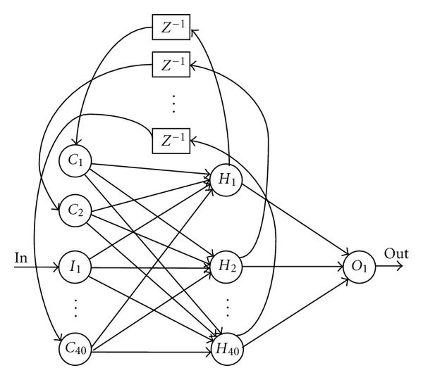
A recurrent neural network (RNN) is a class of artificial neural network where connections between units form a directed cycle. This creates an internal state of the network which allows it to exhibit dynamic temporal behavior. Unlike feed-forward neural networks, RNNs can use their internal memory to process arbitrary sequences of inputs. This makes them applicable to tasks such as unsegmented connected handwriting recognition or speech recognition.
There are a number of Twitter bots that are created using LSTMs. Some fun examples are (???)(https://twitter.com/DeepDrumpf) and (???)(https://twitter.com/DeepLearnBern) by Brad Hayes from MIT.

5.4.3 Convolutional
A convolutional neural network (CNN, or ConvNet) is a type of feed- forward artificial neural network in which the connectivity pattern between its neurons is inspired by the organization of the animal visual cortex, whose individual neurons are arranged in such a way that they respond to overlapping regions tiling the visual field. Convolutional networks were inspired by biological processes and are variations of multilayer perceptrons designed to use minimal amounts of preprocessing. They have wide applications in image and video recognition, recommender systems and natural language processing.
Some creative application of CNNs are DeepDream images and Neural Style Transfer.

5.5 Visualizing Neural Nets

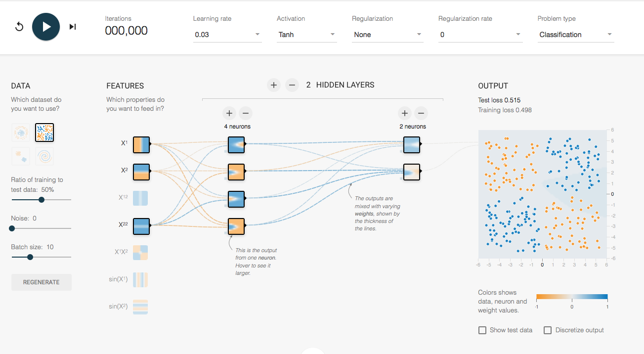
http://playground.tensorflow.org is a website where you can tweak and visualize neural networks.
5.6 Deep Learning Software in R
For the purposes of this tutorial, we will review CPU-based deep learning packages in R that support numeric, tabular data (data frames). There is deep learning software that supports image data directly, but we will not cover those features in this tutorial. The demos below will train a fully-connected, feed- forward ANN (aka mutilayer perceptron) using the mxnet and h2o R packages. Also worth noting are two other Deep Learning packages in R, deepnet and darch (which I don’t have much experience with).
5.6.1 MXNet
Authors: Tianqi Chen, Qiang Kou (KK), et. al.
Backend: C++
MXNet is deep neural net implementation by the same authors as xgboost, and a part of the same umbrella project called DMLC (Distributed Machine Learning Community). The MXNet R package brings flexible and efficient GPU computing and state-of-art deep learning to R.
Features:
- It enables you to write seamless tensor/matrix computation with multiple GPUs in R.
- Distributed computation.
- Read image files directly.
- Offers both a simplified and complex interface for architecting networks.
- Supports mulit-layer feed-forward ANNs (aka. multi-layer perceptrons (MLP)).
- Supports Convolutional Neural Networks (CNN) – good for image recognition.
- Supports Long Short-term memory (LSTM), a type of Recurrent Neural Network (RNN) – good for sequence learning, (e.g. speech, text).
- License: BSD
MXNet Example code below modified from: http://www.r-bloggers.com/deep-learning- with-mxnetr/ The example below contains the canonical 60k/10k MNIST train/test files as opposed to the Kaggle version in the blog post.
# Install pre-build CPU-based mxnet package (no GPU support)
# install.packages("drat")
# drat:::addRepo("dmlc")
# cran <- getOption("repos")
# cran["dmlc"] <- "https://s3-us-west-2.amazonaws.com/apache-mxnet/R/CRAN/"
# options(repos = cran)
# install.packages("mxnet",dependencies = T)library(mxnet)# Data load & preprocessing
## load training data https://h2o-public-test-data.s3.amazonaws.com/bigdata/laptop/mnist/train.csv.gz
train <- data.table::fread("data/mnist_train.csv")
##
Read 66.7% of 60000 rows
Read 60000 rows and 785 (of 785) columns from 0.102 GB file in 00:00:03
## load test data https://h2o-public-test-data.s3.amazonaws.com/bigdata/laptop/mnist/test.csv.gz
test <- data.table::fread("data/mnist_test.csv")
train <- data.matrix(train)
test <- data.matrix(test)
train <- data.matrix(train)
test <- data.matrix(test)
train_x <- train[,-785]
train_y <- train[,785]
test_x <- test[,-785]
test_y <- test[,785]
# lineraly transform it into [0,1]
# transpose input matrix to npixel x nexamples (format expected by mxnet)
train_x <- t(train_x/255)
test_x <- t(test_x/255)
#see that the number of each digit is fairly even
table(train_y)
## train_y
## 0 1 2 3 4 5 6 7 8 9
## 5923 6742 5958 6131 5842 5421 5918 6265 5851 5949# Configure the structure of the network
# in mxnet use its own data type symbol to configure the network
data <- mx.symbol.Variable("data")
# set the first hidden layer where data is the input, name and number of hidden neurons
fc1 <- mx.symbol.FullyConnected(data, name = "fc1", num_hidden = 128)
# set the activation which takes the output from the first hidden layer fc1
act1 <- mx.symbol.Activation(fc1, name = "relu1", act_type = "relu")
# second hidden layer takes the result from act1 as the input, name and number of hidden neurons
fc2 <- mx.symbol.FullyConnected(act1, name = "fc2", num_hidden = 64)
# second activation which takes the output from the second hidden layer fc2
act2 <- mx.symbol.Activation(fc2, name = "relu2", act_type = "relu")
# this is the output layer where number of nuerons is set to 10 because there's only 10 digits
fc3 <- mx.symbol.FullyConnected(act2, name = "fc3", num_hidden = 10)
# finally set the activation to softmax to get a probabilistic prediction
softmax <- mx.symbol.SoftmaxOutput(fc3, name = "sm")# set which device to use before we start the computation
# assign cpu to mxnet
devices <- mx.cpu()
# set seed to control the random process in mxnet
mx.set.seed(0)
# train the nueral network
model <- mx.model.FeedForward.create(
softmax,
X = train_x,
y = train_y,
ctx = devices,
num.round = 10,
array.batch.size = 100,
learning.rate = 0.07,
momentum = 0.9,
eval.metric = mx.metric.accuracy,
initializer = mx.init.uniform(0.07),
epoch.end.callback = mx.callback.log.train.metric(100)
)# make a prediction
preds <- predict(model, test_x)
dim(preds)
## [1] 10 10000
## [1] 10 10000
# matrix with 10000 rows and 10 columns containing the classification probabilities from the output layer
# use max.col to extract the maximum label for each row
pred_label <- max.col(t(preds)) - 1
table(pred_label)
## pred_label
## 0 1 2 3 4 5 6 7 8 9
## 1004 1140 1018 1029 929 880 946 1022 981 1051
# Compute accuracy
acc <- sum(test_y == pred_label)/length(test_y)
print(acc)
## [1] 0.977MXNet also has a simplified api, mx.mlp(), which provides a more generic interface compared to the network construction procedure above.
5.6.2 h2o
Authors: Arno Candel, H2O.ai contributors
Backend: Java
H2O Deep Learning builds a feed-forward multilayer artificial neural network on an distributed H2O data frame.
Features:
- Distributed and parallelized computation on either a single node or a multi- node cluster.
- Data-distributed, which means the entire dataset does not need to fit into memory on a single node.
- Uses HOGWILD! for fast computation.
- Simplified network building interface.
- Fully connected, feed-forward ANNs only (CNNs and LSTMs in development).
- CPU only (GPU interface in development).
- Automatic early stopping based on convergence of user-specied metrics to user- specied relative tolerance.
- Support for exponential families (Poisson, Gamma, Tweedie) and loss functions in addition to binomial (Bernoulli), Gaussian and multinomial distributions, such as Quantile regression (including Laplace).
- Grid search for hyperparameter optimization and model selection.
- Apache 2.0 Licensed.
- Model export in plain Java code for deployment in production environments.
- GUI for training & model eval/viz (H2O Flow).
library(h2o)
h2o.init(nthreads = -1)  # This means nthreads = num available cores
##
## H2O is not running yet, starting it now...
##
## Note:  In case of errors look at the following log files:
##     /var/folders/ws/qs4y2bnx1xs_4y9t0zbdjsvh0000gn/T//Rtmpo3M4DD/h2o_bradboehmke_started_from_r.out
##     /var/folders/ws/qs4y2bnx1xs_4y9t0zbdjsvh0000gn/T//Rtmpo3M4DD/h2o_bradboehmke_started_from_r.err
##
##
## Starting H2O JVM and connecting: .. Connection successful!
##
## R is connected to the H2O cluster:
##     H2O cluster uptime:         2 seconds 643 milliseconds
##     H2O cluster timezone:       America/New_York
##     H2O data parsing timezone:  UTC
##     H2O cluster version:        3.18.0.4
##     H2O cluster version age:    28 days, 3 hours and 13 minutes
##     H2O cluster name:           H2O_started_from_R_bradboehmke_ygp041
##     H2O cluster total nodes:    1
##     H2O cluster total memory:   1.78 GB
##     H2O cluster total cores:    4
##     H2O cluster allowed cores:  4
##     H2O cluster healthy:        TRUE
##     H2O Connection ip:          localhost
##     H2O Connection port:        54321
##     H2O Connection proxy:       NA
##     H2O Internal Security:      FALSE
##     H2O API Extensions:         XGBoost, Algos, AutoML, Core V3, Core V4
##     R Version:                  R version 3.4.4 (2018-03-15)
# Data load & preprocessing
train <- h2o.importFile("data/mnist_train.csv")
##
|
| | 0%
|
|================================================= | 75%
|
|=================================================================| 100%
test <- h2o.importFile("data/mnist_test.csv")
##
|
| | 0%
|
|================ | 25%
|
|=================================================================| 100%
# Specify the response and predictor columns
y <- "C785"
x <- setdiff(names(train), y)
# We encode the response column as categorical for multinomial classification
train[,y] <- as.factor(train[,y])
test[,y] <- as.factor(test[,y])# Train an H2O Deep Learning model
model <- h2o.deeplearning(
x = x,
y = y,
training_frame = train,
sparse = TRUE, #speed-up on sparse data (like MNIST)
distribution = "multinomial",
activation = "Rectifier",
hidden = c(128,64),
epochs = 10
)
##
|
| | 0%
|
|= | 2%
|
|== | 3%
|
|=== | 5%
|
|==== | 7%
|
|====== | 8%
|
|======= | 10%
|
|======== | 12%
|
|========= | 14%
|
|========== | 15%
|
|=========== | 17%
|
|============ | 19%
|
|============= | 20%
|
|============== | 22%
|
|=============== | 24%
|
|================= | 25%
|
|================== | 27%
|
|=================== | 29%
|
|==================== | 31%
|
|===================== | 32%
|
|====================== | 34%
|
|======================= | 36%
|
|======================== | 37%
|
|========================= | 39%
|
|========================== | 41%
|
|============================ | 42%
|
|============================= | 44%
|
|============================== | 46%
|
|=============================== | 48%
|
|================================ | 49%
|
|================================= | 51%
|
|================================== | 53%
|
|=================================== | 54%
|
|==================================== | 56%
|
|====================================== | 58%
|
|======================================= | 59%
|
|======================================== | 61%
|
|========================================= | 63%
|
|========================================== | 65%
|
|=========================================== | 66%
|
|============================================ | 68%
|
|============================================= | 70%
|
|============================================== | 71%
|
|=============================================== | 73%
|
|================================================= | 75%
|
|================================================== | 76%
|
|=================================================== | 78%
|
|==================================================== | 80%
|
|===================================================== | 82%
|
|====================================================== | 83%
|
|======================================================= | 85%
|
|======================================================== | 87%
|
|========================================================= | 88%
|
|=========================================================== | 90%
|
|============================================================ | 92%
|
|============================================================= | 93%
|
|============================================================== | 95%
|
|=============================================================== | 97%
|
|================================================================ | 99%
|
|=================================================================| 100%# Get model performance on a test set
perf <- h2o.performance(model, test)
# Or get the preds directly and compute classification accuracy
preds <- h2o.predict(model, newdata = test)
##
|
| | 0%
|
|=================================================================| 100%
acc <- sum(test[,y] == preds$predict)/nrow(test)
print(acc)
## [1] 0.9724# good practice
h2o.shutdown(prompt = FALSE)
## [1] TRUE