Chapter 4 Generalized Linear Models (GLM)

Image Source: Wikipedia
4.1 Introduction
Linear Models are one of the oldest and most well known statistical prediction algorithms which nowdays is often categorized as a “machine learning algorithm.” Generalized LinearModels (GLMs) are are a framework for modeling a response variable \(y\) that is bounded or discrete. Generalized linear models allow for an arbitrary link function \(g\) that relates the mean of the response variable to the predictors, i.e. \(E(y) = g(β′x)\). The link function is often related to the distribution of the response, and in particular it typically has the effect of transforming between, \((-\infty ,\infty )\), the range of the linear predictor, and the range of the response variable (e.g. \([0,1]\)). [1]
Therefore, GLMs allow for response variables that have error distribution models other than a normal distribution. Some common examples of GLMs are:
- Poisson regression for count data.
- Logistic regression and probit regression for binary data.
- Multinomial logistic regression and multinomial probit regression for categorical data.
- Ordered probit regression for ordinal data.
4.2 Linear Models
In a linear model, given a vector of inputs, \(X^T = (X_1, X_2, ..., X_p)\), we predict the output \(Y\) via the model:
\[\hat{Y} = \hat{\beta}_0 + \sum_{j=1}^p X_j \hat{\beta}_j\]
The term \(\hat{\beta}_0\) is the intercept, also known as the bias in machine learning. Often it is convenient to include the constant variable \(1\) in \(X\), include \(\beta_0\) in the vector of coefficients \(\hat{\beta}\), and then write the linear model in vector form as an inner product,
\[\hat{Y} = X^T\hat{\beta},\]
where \(X^T\) denotes the transpose of the design matrix. We will review the case where \(Y\) is a scalar, however, in general \(Y\) can have more than one dimension. Viewed as a function over the \(p\)-dimensional input space, \(f(X) = X^T\beta\) is linear, and the gradient, \(f′(X) = \beta\), is a vector in input space that points in the steepest uphill direction.
4.2.1 Ordinary Least Squares (OLS)
There are many different methods to fitting a linear model, but the most simple and popular method is Ordinary LeastSquares (OLS). The OLS method minimizes the residual sum ofsquares (RSS), and leads to a closed-form expression for the estimated value of the unknown parameter \(\beta\).
\[RSS(\beta) = \sum_{i=1}^n (y_i - x_i^T\beta)^2\]
\(RSS(\beta)\) is a quadradic function of the parameters, and hence its minimum always exists, but may not be unique. The solution is easiest to characterize in matrix notation:
\[RSS(\beta) = (\boldsymbol{y} - \boldsymbol{X}\beta)^T(\boldsymbol{y} - \boldsymbol{X}\beta)\]
where \(\boldsymbol{X}\) is an \(n \times p\) matrix with each row an input vector, and \(\boldsymbol{y}\) is a vector of length \(n\) representing the response in the training set. Differentiating with respect to \(\beta\), we get the normal equations,
\[\boldsymbol{X}^T(\boldsymbol{y} - \boldsymbol{X}\beta) = 0\]
If \(\boldsymbol{X}^T\boldsymbol{X}\) is nonsingular, then the unique solution is given by:
\[\hat{\beta} = (\boldsymbol{X}^T\boldsymbol{X})^{-1}\boldsymbol{X}^T\boldsymbol{y}\]
The fitted value at the \(i^{th}\) input, \(x_i\) is \(\hat{y}_i = \hat{y}(x_i) = x_i^T\hat{\beta}\). To solve this equation for \(\beta\), we must invert a matrix, \(\boldsymbol{X}^T\boldsymbol{X}\), however it can be computationally expensive to invert this matrix directly. There are computational shortcuts for solving the normal equations available via QR or Cholesky decomposition. When dealing with large training sets, it is useful to have an understanding of the underlying computational methods in the software that you are using. Some GLM software implementations may not utilize all available computational shortcuts, costing you extra time to train your GLMs, or require you to upgrade the memory on your machine.
4.3 Regularization
http://web.stanford.edu/~hastie/Papers/glmpath.pdf
4.3.1 Ridge Regression
Consider a sample consisting of \(n\) cases, each of which consists of \(p\) covariates and a single outcome. Let \(y_i\) be the outcome and \(X_i := ( x_1 , x_2 , … , x_p)^T\).
Then the objective of Ridge is to solve:
\[{\displaystyle \min _{\beta }\left\{{\frac {1}{N}}\sum _{i=1}^{N}\left(y_{i}-\beta_0 - \sum_{j=1}^p x_{ij}\beta_j \right)^{2}\right\}{\text{ subject to }}\sum _{j=1}^{p}\beta _{j}^2 \leq t.}\]
Here \(t\) is a prespecified free parameter that determines the amount of regularization. Ridge is also called \(\ell_2\) regularization.
4.3.2 Lasso Regression
Lasso (least absolute shrinkage and selection operator) (also Lasso or LASSO) is a regression analysis method that performs both variable selection and regularization in order to enhance the prediction accuracy and interpretability of the statistical model it produces.
- It was introduced by Robert Tibshirani in 1996 based on Leo Breiman’s Nonnegative Garrote.
- Lasso conveniently performs coefficient shrinkage comparable to the ridge regression as well as variable selection by reducing coefficients to zero.
- By sacrificing a small amount of bias in the predicted response variable in order to decrease variance, the lasso achieves improved predictive accuracy compared with ordinary least squares (OLS) models, particularly with data containing highly correlated predictor variables or in over determined data where \(p>n\).
Then the objective of Lasso is to solve:
\[{\displaystyle \min _{\beta }\left\{{\frac {1}{N}}\sum _{i=1}^{N}\left(y_{i}-\beta_0 - \sum_{j=1}^p x_{ij}\beta_j \right)^{2}\right\}{\text{ subject to }}\sum _{j=1}^{p}|\beta _{j}| \leq t.}\]
Here \(t\) is a prespecified free parameter that determines the amount of regularization. Lasso is also called \(\ell_1\) regularization.
4.3.3 Elastic Net
Elastic Net regularization is a simple blend of Lasso and Ridge regularization. In software, this is typically controlled by an alpha parameter in between 0 and 1, where:
alpha = 0.0is Ridge regressionalpha = 0.5is a 50/50 blend of Ridge/Lasso regressionalpha = 1.0is Lasso regression
4.4 Other Solvers
GLM models are trained by finding the set of parameters that maximizes the likelihood of the data. For the Gaussian family, maximum likelihood consists of minimizing the mean squared error. This has an analytical solution and can be solved with a standard method of least squares. This is also applicable when the \(\ell_2\) penalty is added to the optimization. For all other families and when the \(\ell_1\) penalty is included, the maximum likelihood problem has no analytical solution. Therefore an iterative method such as IRLSM, L-BFGS, the Newton method, or gradient descent, must be used.
4.4.1 Iteratively Re-weighted Least Squares (IRLS)
The IRLS method is used to solve certain optimization problems with objective functions of the form:
\[{\underset {{\boldsymbol \beta }}{\operatorname {arg\,min}}}\sum _{{i=1}}^{n}{\big |}y_{i}-f_{i}({\boldsymbol \beta }){\big |}^{p},\]
by an iterative method in which each step involves solving a weighted least squares problem of the form:
\[{\boldsymbol \beta }^{{(t+1)}}={\underset {{\boldsymbol \beta }}{\operatorname {arg\,min}}}\sum _{{i=1}}^{n}w_{i}({\boldsymbol \beta }^{{(t)}}){\big |}y_{i}-f_{i}({\boldsymbol \beta }){\big |}^{2}.\]
IRLS is used to find the maximum likelihood estimates of a generalized linear model as a way of mitigating the influence of outliers in an otherwise normally-distributed data set. For example, by minimizing the least absolute error rather than the least square error.
One of the advantages of IRLS over linear programming and convex programming is that it can be used with Gauss-Newton and Levenberg-Marquardt numerical algorithms.
The IRL1 algorithm solves a sequence of non-smooth weighted \(\ell_1\)-minimization problems, and hence can be seen as the non-smooth counterpart to the IRLS algorithm.
4.4.2 Iteratively Re-weighted Least Squares with ADMM
The IRLS method with alternating direction method of multipliers (ADMM) inner solver as described in Distributed Optimization and Statistical Learning via the Alternating Direction Method of Multipliers by Boyd et. al to deal with the \(\ell_1\) penalty. ADMM is an algorithm that solves convex optimization problems by breaking them into smaller pieces, each of which are then easier to handle. Every iteration of the algorithm consists of following steps:
- Generate weighted least squares problem based on previous solution, i.e. vector of weights w and response z.
- Compute the weighted Gram matrix XT WX and XT z vector
- Decompose the Gram matrix (Cholesky decomposition) and apply ADMM solver to solve the \(\ell_1\) penalized least squares problem.
In the H2O GLM implementation, steps 1 and 2 are performed distributively, and Step 3 is computed in parallel on a single node. The Gram matrix appraoch is very efficient for tall and narrow datasets when running lamnda search with a sparse solution.
4.4.3 Cyclical Coordinate Descent
The IRLS method can also use cyclical coordinate descent in it’s inner loop (as opposed to ADMM). The glmnet package uses cyclical coordinate descent which successively optimizes the objective function over each parameter with others fixed, and cycles repeatedly until convergence.
Cyclical coordinate descent methods are a natural approach for solving convex problems with \(\ell_1\) or \(\ell_2\) constraints, or mixtures of the two (elastic net). Each coordinate-descent step is fast, with an explicit formula for each coordinate-wise minimization. The method also exploits the sparsity of the model, spending much of its time evaluating only inner products for variables with non-zero coefficients.
4.4.4 L-BFGS
Limited-memory BFGS (L-BFGS) is an optimization algorithm in the family of quasi-Newton methods that approximates the Broyden–Fletcher–Goldfarb–Shanno (BFGS) algorithm using a limited amount of computer memory. Due to its resulting linear memory requirement, the L-BFGS method is particularly well suited for optimization problems with a large number of variables. The method is popular among “big data” GLM implementations such as h2o::h2o.glm() (one of two available solvers) and SparkR::glm(). The L-BFGS-B algorithm is an extension of the L-BFGS algorithm to handle simple bounds on the model.
4.5 Data Preprocessing
In order for the coefficients to be easily interpretable, the features must be centered and scaled (aka “normalized”). Many software packages will allow the direct input of categorical/factor columns in the training frame, however internally any categorical columns will be expaded into binary indicator variables. The caret package offers a handy utility function, caret::dummyVars (), for dummy/indicator expansion if you need to do this manually.
Missing data will need to be imputed, otherwise in many GLM packages, those rows will simply be omitted from the training set at train time. For example, in the stats::glm() function there is an na.action argument which allows the user to do one of the three options:
- na.omit and na.exclude: observations are removed if they contain any missing values; if na.exclude is used some functions will pad residuals and predictions to the correct length by inserting NAs for omitted cases.
- na.pass: keep all data, including NAs
- na.fail: returns the object only if it contains no missing values
Other GLM implementations such as h2o::glm() will impute the mean automatically (in both training and test data), unless specified by the user.
4.6 GLM Software in R
There is an implementation of the standard GLM (no regularization) in the built- in “stats” package in R called glm.
4.6.1 glm
Authors: The original R implementation of glm was written by Simon Davies working for Ross Ihaka at the University of Auckland, but has since been extensively re-written by members of the R Core team. The design was inspired by the S function of the same name described in Hastie & Pregibon (1992).
Backend: Fortran
4.6.1.1 Example Linear Regression with glm()
#install.packages("caret")
library(caret)
data("Sacramento")

# Split the data into a 70/25% train/test sets
set.seed(1)
idxs <- caret::createDataPartition(y = Sacramento$price, p = 0.75)[[1]]
train <- Sacramento[idxs,]
test <- Sacramento[-idxs,]
# Fit the GLM
fit <- glm(
price ~ .,
data = train,
family = gaussian()
)
summary(fit)
##
## Call:
## glm(formula = price ~ ., family = gaussian(), data = train)
##
## Deviance Residuals:
## Min 1Q Median 3Q Max
## -269404 -39233 -6677 27418 279476
##
## Coefficients: (32 not defined because of singularities)
## Estimate Std. Error t value Pr(>|t|)
## (Intercept) 7.434e+06 1.931e+07 0.385 0.700365
## cityAUBURN 1.450e+05 7.163e+04 2.024 0.043348 *
## cityCAMERON_PARK 3.497e+04 6.341e+04 0.551 0.581536
## cityCARMICHAEL 8.019e+04 2.699e+04 2.971 0.003078 **
## cityCITRUS_HEIGHTS -8.352e+03 2.222e+04 -0.376 0.707161
## cityCOOL 1.300e+05 1.015e+05 1.281 0.200691
## cityEL_DORADO 3.534e+04 1.061e+05 0.333 0.739141
## cityEL_DORADO_HILLS 1.243e+05 5.417e+04 2.295 0.022047 *
## cityELK_GROVE -6.302e+04 5.984e+04 -1.053 0.292688
## cityELVERTA -5.559e+04 5.066e+04 -1.097 0.272929
## cityFAIR_OAKS 6.136e+04 3.307e+04 1.855 0.064008 .
## cityFOLSOM 1.056e+05 4.168e+04 2.533 0.011540 *
## cityFORESTHILL 7.605e+04 1.283e+05 0.593 0.553518
## cityGALT -9.711e+04 8.547e+04 -1.136 0.256354
## cityGOLD_RIVER 3.459e+04 6.240e+04 0.554 0.579555
## cityGRANITE_BAY 3.217e+05 7.939e+04 4.053 5.70e-05 ***
## cityGREENWOOD 7.445e+04 1.119e+05 0.665 0.506249
## cityLINCOLN 3.605e+04 3.989e+04 0.904 0.366484
## cityLOOMIS 3.754e+05 6.367e+04 5.896 6.08e-09 ***
## cityMATHER -8.306e+04 7.679e+04 -1.082 0.279856
## cityMEADOW_VISTA 1.221e+05 1.060e+05 1.153 0.249537
## cityNORTH_HIGHLANDS -3.655e+04 2.425e+04 -1.507 0.132220
## cityORANGEVALE 5.875e+04 3.518e+04 1.670 0.095465 .
## cityPLACERVILLE 1.271e+05 9.188e+04 1.384 0.166998
## cityPOLLOCK_PINES 3.648e+04 1.291e+05 0.283 0.777580
## cityRANCHO_CORDOVA -6.894e+04 4.502e+04 -1.531 0.126222
## cityRANCHO_MURIETA -1.675e+05 8.849e+04 -1.893 0.058780 .
## cityRIO_LINDA -2.221e+04 3.001e+04 -0.740 0.459428
## cityROCKLIN 9.179e+04 3.562e+04 2.577 0.010205 *
## cityROSEVILLE 9.536e+04 2.678e+04 3.560 0.000398 ***
## citySACRAMENTO 1.203e+05 4.113e+04 2.926 0.003561 **
## cityWALNUT_GROVE 4.904e+04 1.173e+05 0.418 0.676124
## cityWEST_SACRAMENTO -7.501e+04 6.405e+04 -1.171 0.242019
## cityWILTON 1.265e+05 7.234e+04 1.749 0.080744 .
## zipz95608 NA NA NA NA
## zipz95610 7.732e+03 3.056e+04 0.253 0.800363
## zipz95614 NA NA NA NA
## zipz95621 NA NA NA NA
## zipz95623 NA NA NA NA
## zipz95624 -1.452e+03 2.038e+04 -0.071 0.943237
## zipz95626 NA NA NA NA
## zipz95628 NA NA NA NA
## zipz95630 NA NA NA NA
## zipz95631 NA NA NA NA
## zipz95632 NA NA NA NA
## zipz95635 NA NA NA NA
## zipz95648 NA NA NA NA
## zipz95650 NA NA NA NA
## zipz95655 NA NA NA NA
## zipz95660 NA NA NA NA
## zipz95661 2.926e+04 3.994e+04 0.733 0.464062
## zipz95662 NA NA NA NA
## zipz95667 NA NA NA NA
## zipz95670 5.343e+04 3.267e+04 1.635 0.102495
## zipz95673 NA NA NA NA
## zipz95677 1.607e+04 4.510e+04 0.356 0.721739
## zipz95678 -4.077e+04 2.838e+04 -1.437 0.151329
## zipz95682 NA NA NA NA
## zipz95683 NA NA NA NA
## zipz95690 NA NA NA NA
## zipz95691 NA NA NA NA
## zipz95693 NA NA NA NA
## zipz95722 NA NA NA NA
## zipz95726 NA NA NA NA
## zipz95742 NA NA NA NA
## zipz95746 NA NA NA NA
## zipz95747 NA NA NA NA
## zipz95757 1.339e+04 1.874e+04 0.715 0.475149
## zipz95758 NA NA NA NA
## zipz95762 NA NA NA NA
## zipz95765 NA NA NA NA
## zipz95811 1.067e+05 7.624e+04 1.400 0.162053
## zipz95814 -7.275e+04 6.049e+04 -1.203 0.229549
## zipz95815 -1.940e+05 3.691e+04 -5.256 2.02e-07 ***
## zipz95816 -2.631e+03 4.872e+04 -0.054 0.956956
## zipz95817 -1.662e+05 4.612e+04 -3.605 0.000337 ***
## zipz95818 -5.284e+04 4.452e+04 -1.187 0.235783
## zipz95819 1.074e+05 5.104e+04 2.104 0.035800 *
## zipz95820 -1.712e+05 3.770e+04 -4.540 6.73e-06 ***
## zipz95821 -9.943e+04 4.344e+04 -2.289 0.022420 *
## zipz95822 -1.762e+05 4.333e+04 -4.066 5.39e-05 ***
## zipz95823 -2.001e+05 4.157e+04 -4.813 1.86e-06 ***
## zipz95824 -2.056e+05 4.097e+04 -5.019 6.77e-07 ***
## zipz95825 -1.386e+05 3.719e+04 -3.727 0.000212 ***
## zipz95826 -1.435e+05 3.811e+04 -3.765 0.000182 ***
## zipz95827 -1.880e+05 4.005e+04 -4.694 3.30e-06 ***
## zipz95828 -2.005e+05 3.935e+04 -5.096 4.60e-07 ***
## zipz95829 -1.802e+05 4.471e+04 -4.030 6.25e-05 ***
## zipz95831 -1.137e+05 5.317e+04 -2.138 0.032914 *
## zipz95832 -2.242e+05 4.891e+04 -4.584 5.52e-06 ***
## zipz95833 -1.549e+05 4.048e+04 -3.827 0.000143 ***
## zipz95834 -1.510e+05 4.150e+04 -3.639 0.000297 ***
## zipz95835 -1.202e+05 4.195e+04 -2.865 0.004309 **
## zipz95838 -1.729e+05 3.648e+04 -4.741 2.64e-06 ***
## zipz95841 -7.757e+04 5.190e+04 -1.495 0.135538
## zipz95842 -1.651e+05 3.921e+04 -4.210 2.93e-05 ***
## zipz95843 NA NA NA NA
## zipz95864 NA NA NA NA
## beds -1.336e+04 5.016e+03 -2.664 0.007926 **
## baths 1.314e+04 6.323e+03 2.078 0.038099 *
## sqft 1.148e+02 7.457e+00 15.388 < 2e-16 ***
## typeMulti_Family 3.034e+04 2.731e+04 1.111 0.266933
## typeResidential 4.665e+04 1.298e+04 3.594 0.000351 ***
## latitude -2.121e+05 1.895e+05 -1.120 0.263319
## longitude -6.519e+03 1.547e+05 -0.042 0.966399
## ---
## Signif. codes: 0 '***' 0.001 '**' 0.01 '*' 0.05 '.' 0.1 ' ' 1
##
## (Dispersion parameter for gaussian family taken to be 4622177625)
##
## Null deviance: 1.2350e+13 on 699 degrees of freedom
## Residual deviance: 2.8981e+12 on 627 degrees of freedom
## AIC: 17635
##
## Number of Fisher Scoring iterations: 2# Predict on the test set
pred <- predict(fit, newdata = test)
## Error in model.frame.default(Terms, newdata, na.action = na.action, xlev = object$xlevels): factor city has new levels DIAMOND_SPRINGS, GARDEN_VALLEY, PENRYNAbove we have a slight issue. The city column has new factor levels in the test set that were not present in the training set. Even though the train and test data frames originated from a single data frame, Sacramento, and therefore have identical factor levels, we still run into this problem. Let’s take a closer look at the factor levels to see what’s going on:
str(train)
## 'data.frame':    700 obs. of  9 variables:
##  $ city     : Factor w/ 37 levels "ANTELOPE","AUBURN",..: 34 34 34 34 34 29 31 34 34 34 ...
##  $ zip      : Factor w/ 68 levels "z95603","z95608",..: 52 44 44 53 65 24 25 44 51 66 ...
##  $ beds     : int  3 2 2 2 3 2 3 1 3 2 ...
##  $ baths    : num  1 1 1 1 1 2 2 1 1 2 ...
##  $ sqft     : int  1167 796 852 797 1122 941 1146 871 1020 1022 ...
##  $ type     : Factor w/ 3 levels "Condo","Multi_Family",..: 3 3 3 3 1 1 3 3 3 3 ...
##  $ price    : int  68212 68880 69307 81900 89921 94905 98937 106852 107502 108750 ...
##  $ latitude : num  38.5 38.6 38.6 38.5 38.7 ...
## $ longitude: num -121 -121 -121 -121 -121 ...str(test)
## 'data.frame': 232 obs. of 9 variables:
## $ city : Factor w/ 37 levels "ANTELOPE","AUBURN",..: 34 34 34 34 34 1 34 24 11 10 ...
## $ zip : Factor w/ 68 levels "z95603","z95608",..: 64 66 49 64 52 67 57 19 9 8 ...
## $ beds : int 2 3 3 3 3 3 3 3 3 3 ...
## $ baths : num 1 2 1 2 2 2 2 2 2 2 ...
## $ sqft : int 836 1104 1177 909 1289 1088 1248 1152 1116 1056 ...
## $ type : Factor w/ 3 levels "Condo","Multi_Family",..: 3 3 3 3 3 3 3 3 3 3 ...
## $ price : int 59222 90895 91002 100309 106250 126640 132000 134555 138750 156896 ...
## $ latitude : num 38.6 38.7 38.5 38.6 38.5 ...
## $ longitude: num -121 -121 -121 -121 -121 ...Although train and test have identical structure, not all the levels are represented in the training data. To validate this, let’s take a look at the actual unique levels that were used in the model:
# Check the number of levels in the model features
sapply(fit$xlevels, function(x) print(length(x)))
## [1] 34
## [1] 65
## [1] 3
## city  zip type
##   34   65    3
We can manually fix this by updating the xlevels element of the model. We have the same issue with zip, so we should go ahead and manually update that as well.
# Update factor levels so that prediction works
fit$xlevels[["city"]] <- union(fit$xlevels[["city"]], levels(test$city))
fit$xlevels[["zip"]] <- union(fit$xlevels[["zip"]], levels(test$zip))
# Predict on the test set
pred <- predict(fit, newdata = test)
summary(fit)
##
## Call:
## glm(formula = price ~ ., family = gaussian(), data = train)
##
## Deviance Residuals:
## Min 1Q Median 3Q Max
## -269404 -39233 -6677 27418 279476
##
## Coefficients: (32 not defined because of singularities)
## Estimate Std. Error t value Pr(>|t|)
## (Intercept) 7.434e+06 1.931e+07 0.385 0.700365
## cityAUBURN 1.450e+05 7.163e+04 2.024 0.043348 *
## cityCAMERON_PARK 3.497e+04 6.341e+04 0.551 0.581536
## cityCARMICHAEL 8.019e+04 2.699e+04 2.971 0.003078 **
## cityCITRUS_HEIGHTS -8.352e+03 2.222e+04 -0.376 0.707161
## cityCOOL 1.300e+05 1.015e+05 1.281 0.200691
## cityEL_DORADO 3.534e+04 1.061e+05 0.333 0.739141
## cityEL_DORADO_HILLS 1.243e+05 5.417e+04 2.295 0.022047 *
## cityELK_GROVE -6.302e+04 5.984e+04 -1.053 0.292688
## cityELVERTA -5.559e+04 5.066e+04 -1.097 0.272929
## cityFAIR_OAKS 6.136e+04 3.307e+04 1.855 0.064008 .
## cityFOLSOM 1.056e+05 4.168e+04 2.533 0.011540 *
## cityFORESTHILL 7.605e+04 1.283e+05 0.593 0.553518
## cityGALT -9.711e+04 8.547e+04 -1.136 0.256354
## cityGOLD_RIVER 3.459e+04 6.240e+04 0.554 0.579555
## cityGRANITE_BAY 3.217e+05 7.939e+04 4.053 5.70e-05 ***
## cityGREENWOOD 7.445e+04 1.119e+05 0.665 0.506249
## cityLINCOLN 3.605e+04 3.989e+04 0.904 0.366484
## cityLOOMIS 3.754e+05 6.367e+04 5.896 6.08e-09 ***
## cityMATHER -8.306e+04 7.679e+04 -1.082 0.279856
## cityMEADOW_VISTA 1.221e+05 1.060e+05 1.153 0.249537
## cityNORTH_HIGHLANDS -3.655e+04 2.425e+04 -1.507 0.132220
## cityORANGEVALE 5.875e+04 3.518e+04 1.670 0.095465 .
## cityPLACERVILLE 1.271e+05 9.188e+04 1.384 0.166998
## cityPOLLOCK_PINES 3.648e+04 1.291e+05 0.283 0.777580
## cityRANCHO_CORDOVA -6.894e+04 4.502e+04 -1.531 0.126222
## cityRANCHO_MURIETA -1.675e+05 8.849e+04 -1.893 0.058780 .
## cityRIO_LINDA -2.221e+04 3.001e+04 -0.740 0.459428
## cityROCKLIN 9.179e+04 3.562e+04 2.577 0.010205 *
## cityROSEVILLE 9.536e+04 2.678e+04 3.560 0.000398 ***
## citySACRAMENTO 1.203e+05 4.113e+04 2.926 0.003561 **
## cityWALNUT_GROVE 4.904e+04 1.173e+05 0.418 0.676124
## cityWEST_SACRAMENTO -7.501e+04 6.405e+04 -1.171 0.242019
## cityWILTON 1.265e+05 7.234e+04 1.749 0.080744 .
## zipz95608 NA NA NA NA
## zipz95610 7.732e+03 3.056e+04 0.253 0.800363
## zipz95614 NA NA NA NA
## zipz95621 NA NA NA NA
## zipz95623 NA NA NA NA
## zipz95624 -1.452e+03 2.038e+04 -0.071 0.943237
## zipz95626 NA NA NA NA
## zipz95628 NA NA NA NA
## zipz95630 NA NA NA NA
## zipz95631 NA NA NA NA
## zipz95632 NA NA NA NA
## zipz95635 NA NA NA NA
## zipz95648 NA NA NA NA
## zipz95650 NA NA NA NA
## zipz95655 NA NA NA NA
## zipz95660 NA NA NA NA
## zipz95661 2.926e+04 3.994e+04 0.733 0.464062
## zipz95662 NA NA NA NA
## zipz95667 NA NA NA NA
## zipz95670 5.343e+04 3.267e+04 1.635 0.102495
## zipz95673 NA NA NA NA
## zipz95677 1.607e+04 4.510e+04 0.356 0.721739
## zipz95678 -4.077e+04 2.838e+04 -1.437 0.151329
## zipz95682 NA NA NA NA
## zipz95683 NA NA NA NA
## zipz95690 NA NA NA NA
## zipz95691 NA NA NA NA
## zipz95693 NA NA NA NA
## zipz95722 NA NA NA NA
## zipz95726 NA NA NA NA
## zipz95742 NA NA NA NA
## zipz95746 NA NA NA NA
## zipz95747 NA NA NA NA
## zipz95757 1.339e+04 1.874e+04 0.715 0.475149
## zipz95758 NA NA NA NA
## zipz95762 NA NA NA NA
## zipz95765 NA NA NA NA
## zipz95811 1.067e+05 7.624e+04 1.400 0.162053
## zipz95814 -7.275e+04 6.049e+04 -1.203 0.229549
## zipz95815 -1.940e+05 3.691e+04 -5.256 2.02e-07 ***
## zipz95816 -2.631e+03 4.872e+04 -0.054 0.956956
## zipz95817 -1.662e+05 4.612e+04 -3.605 0.000337 ***
## zipz95818 -5.284e+04 4.452e+04 -1.187 0.235783
## zipz95819 1.074e+05 5.104e+04 2.104 0.035800 *
## zipz95820 -1.712e+05 3.770e+04 -4.540 6.73e-06 ***
## zipz95821 -9.943e+04 4.344e+04 -2.289 0.022420 *
## zipz95822 -1.762e+05 4.333e+04 -4.066 5.39e-05 ***
## zipz95823 -2.001e+05 4.157e+04 -4.813 1.86e-06 ***
## zipz95824 -2.056e+05 4.097e+04 -5.019 6.77e-07 ***
## zipz95825 -1.386e+05 3.719e+04 -3.727 0.000212 ***
## zipz95826 -1.435e+05 3.811e+04 -3.765 0.000182 ***
## zipz95827 -1.880e+05 4.005e+04 -4.694 3.30e-06 ***
## zipz95828 -2.005e+05 3.935e+04 -5.096 4.60e-07 ***
## zipz95829 -1.802e+05 4.471e+04 -4.030 6.25e-05 ***
## zipz95831 -1.137e+05 5.317e+04 -2.138 0.032914 *
## zipz95832 -2.242e+05 4.891e+04 -4.584 5.52e-06 ***
## zipz95833 -1.549e+05 4.048e+04 -3.827 0.000143 ***
## zipz95834 -1.510e+05 4.150e+04 -3.639 0.000297 ***
## zipz95835 -1.202e+05 4.195e+04 -2.865 0.004309 **
## zipz95838 -1.729e+05 3.648e+04 -4.741 2.64e-06 ***
## zipz95841 -7.757e+04 5.190e+04 -1.495 0.135538
## zipz95842 -1.651e+05 3.921e+04 -4.210 2.93e-05 ***
## zipz95843 NA NA NA NA
## zipz95864 NA NA NA NA
## beds -1.336e+04 5.016e+03 -2.664 0.007926 **
## baths 1.314e+04 6.323e+03 2.078 0.038099 *
## sqft 1.148e+02 7.457e+00 15.388 < 2e-16 ***
## typeMulti_Family 3.034e+04 2.731e+04 1.111 0.266933
## typeResidential 4.665e+04 1.298e+04 3.594 0.000351 ***
## latitude -2.121e+05 1.895e+05 -1.120 0.263319
## longitude -6.519e+03 1.547e+05 -0.042 0.966399
## ---
## Signif. codes: 0 '***' 0.001 '**' 0.01 '*' 0.05 '.' 0.1 ' ' 1
##
## (Dispersion parameter for gaussian family taken to be 4622177625)
##
## Null deviance: 1.2350e+13 on 699 degrees of freedom
## Residual deviance: 2.8981e+12 on 627 degrees of freedom
## AIC: 17635
##
## Number of Fisher Scoring iterations: 2# Compute model performance on the test set
caret::R2(pred = pred, obs = test$price)
## [1] 0.03715124
caret::RMSE(pred = pred, obs = test$price)
## [1] 71739824.6.2 GLM in caret
Now let’s run the same model using caret’s glm method to get a sense of how much easier it is to use.
# Train a caret glm model
fit <- caret::train(
  form = price ~ .,
  data = train,
  trControl = trainControl(method = "none"),
  method = "glm",
  family = gaussian()
  )

summary(fit$finalModel)
##
## Call:
## NULL
##
## Deviance Residuals:
##     Min       1Q   Median       3Q      Max
## -269404   -39233    -6677    27418   279476
##
## Coefficients: (38 not defined because of singularities)
##                       Estimate Std. Error t value Pr(>|t|)
## (Intercept)          7.434e+06  1.931e+07   0.385 0.700365
## cityAUBURN           1.450e+05  7.163e+04   2.024 0.043348 *
## cityCAMERON_PARK     3.497e+04  6.341e+04   0.551 0.581536
## cityCARMICHAEL       8.019e+04  2.699e+04   2.971 0.003078 **
## cityCITRUS_HEIGHTS  -8.352e+03  2.222e+04  -0.376 0.707161
## cityCOOL             1.300e+05  1.015e+05   1.281 0.200691
## cityDIAMOND_SPRINGS         NA         NA      NA       NA
## cityEL_DORADO        3.534e+04  1.061e+05   0.333 0.739141
## cityEL_DORADO_HILLS  1.243e+05  5.417e+04   2.295 0.022047 *
## cityELK_GROVE       -6.302e+04  5.984e+04  -1.053 0.292688
## cityELVERTA         -5.559e+04  5.066e+04  -1.097 0.272929
## cityFAIR_OAKS        6.136e+04  3.307e+04   1.855 0.064008 .
## cityFOLSOM           1.056e+05  4.168e+04   2.533 0.011540 *
## cityFORESTHILL       7.605e+04  1.283e+05   0.593 0.553518
## cityGALT            -9.711e+04  8.547e+04  -1.136 0.256354
## cityGARDEN_VALLEY           NA         NA      NA       NA
## cityGOLD_RIVER       3.459e+04  6.240e+04   0.554 0.579555
## cityGRANITE_BAY      3.217e+05  7.939e+04   4.053 5.70e-05 ***
## cityGREENWOOD        7.445e+04  1.119e+05   0.665 0.506249
## cityLINCOLN          3.605e+04  3.989e+04   0.904 0.366484
## cityLOOMIS           3.754e+05  6.367e+04   5.896 6.08e-09 ***
## cityMATHER          -8.306e+04  7.679e+04  -1.082 0.279856
## cityMEADOW_VISTA     1.221e+05  1.060e+05   1.153 0.249537
## cityNORTH_HIGHLANDS -3.655e+04  2.425e+04  -1.507 0.132220
## cityORANGEVALE       5.875e+04  3.518e+04   1.670 0.095465 .
## cityPENRYN                  NA         NA      NA       NA
## cityPLACERVILLE      1.271e+05  9.188e+04   1.384 0.166998
## cityPOLLOCK_PINES    3.648e+04  1.291e+05   0.283 0.777580
## cityRANCHO_CORDOVA  -6.894e+04  4.502e+04  -1.531 0.126222
## cityRANCHO_MURIETA  -1.675e+05  8.849e+04  -1.893 0.058780 .
## cityRIO_LINDA       -2.221e+04  3.001e+04  -0.740 0.459428
## cityROCKLIN          9.179e+04  3.562e+04   2.577 0.010205 *
## cityROSEVILLE        9.536e+04  2.678e+04   3.560 0.000398 ***
## citySACRAMENTO       1.203e+05  4.113e+04   2.926 0.003561 **
## cityWALNUT_GROVE     4.904e+04  1.173e+05   0.418 0.676124
## cityWEST_SACRAMENTO -7.501e+04  6.405e+04  -1.171 0.242019
## cityWILTON           1.265e+05  7.234e+04   1.749 0.080744 .
## zipz95608                   NA         NA      NA       NA
## zipz95610            7.732e+03  3.056e+04   0.253 0.800363
## zipz95614                   NA         NA      NA       NA
## zipz95619                   NA         NA      NA       NA
## zipz95621                   NA         NA      NA       NA
## zipz95623                   NA         NA      NA       NA
## zipz95624           -1.452e+03  2.038e+04  -0.071 0.943237
## zipz95626                   NA         NA      NA       NA
## zipz95628                   NA         NA      NA       NA
## zipz95630                   NA         NA      NA       NA
## zipz95631                   NA         NA      NA       NA
## zipz95632                   NA         NA      NA       NA
## zipz95633                   NA         NA      NA       NA
## zipz95635                   NA         NA      NA       NA
## zipz95648                   NA         NA      NA       NA
## zipz95650                   NA         NA      NA       NA
## zipz95655                   NA         NA      NA       NA
## zipz95660                   NA         NA      NA       NA
## zipz95661            2.926e+04  3.994e+04   0.733 0.464062
## zipz95662                   NA         NA      NA       NA
## zipz95663                   NA         NA      NA       NA
## zipz95667                   NA         NA      NA       NA
## zipz95670            5.343e+04  3.267e+04   1.635 0.102495
## zipz95673                   NA         NA      NA       NA
## zipz95677            1.607e+04  4.510e+04   0.356 0.721739
## zipz95678           -4.077e+04  2.838e+04  -1.437 0.151329
## zipz95682                   NA         NA      NA       NA
## zipz95683                   NA         NA      NA       NA
## zipz95690                   NA         NA      NA       NA
## zipz95691                   NA         NA      NA       NA
## zipz95693                   NA         NA      NA       NA
## zipz95722                   NA         NA      NA       NA
## zipz95726                   NA         NA      NA       NA
## zipz95742                   NA         NA      NA       NA
## zipz95746                   NA         NA      NA       NA
## zipz95747                   NA         NA      NA       NA
## zipz95757            1.339e+04  1.874e+04   0.715 0.475149
## zipz95758                   NA         NA      NA       NA
## zipz95762                   NA         NA      NA       NA
## zipz95765                   NA         NA      NA       NA
## zipz95811            1.067e+05  7.624e+04   1.400 0.162053
## zipz95814           -7.275e+04  6.049e+04  -1.203 0.229549
## zipz95815           -1.940e+05  3.691e+04  -5.256 2.02e-07 ***
## zipz95816           -2.631e+03  4.872e+04  -0.054 0.956956
## zipz95817           -1.662e+05  4.612e+04  -3.605 0.000337 ***
## zipz95818           -5.284e+04  4.452e+04  -1.187 0.235783
## zipz95819            1.074e+05  5.104e+04   2.104 0.035800 *
## zipz95820           -1.712e+05  3.770e+04  -4.540 6.73e-06 ***
## zipz95821           -9.943e+04  4.344e+04  -2.289 0.022420 *
## zipz95822           -1.762e+05  4.333e+04  -4.066 5.39e-05 ***
## zipz95823           -2.001e+05  4.157e+04  -4.813 1.86e-06 ***
## zipz95824           -2.056e+05  4.097e+04  -5.019 6.77e-07 ***
## zipz95825           -1.386e+05  3.719e+04  -3.727 0.000212 ***
## zipz95826           -1.435e+05  3.811e+04  -3.765 0.000182 ***
## zipz95827           -1.880e+05  4.005e+04  -4.694 3.30e-06 ***
## zipz95828           -2.005e+05  3.935e+04  -5.096 4.60e-07 ***
## zipz95829           -1.802e+05  4.471e+04  -4.030 6.25e-05 ***
## zipz95831           -1.137e+05  5.317e+04  -2.138 0.032914 *
## zipz95832           -2.242e+05  4.891e+04  -4.584 5.52e-06 ***
## zipz95833           -1.549e+05  4.048e+04  -3.827 0.000143 ***
## zipz95834           -1.510e+05  4.150e+04  -3.639 0.000297 ***
## zipz95835           -1.202e+05  4.195e+04  -2.865 0.004309 **
## zipz95838           -1.729e+05  3.648e+04  -4.741 2.64e-06 ***
## zipz95841           -7.757e+04  5.190e+04  -1.495 0.135538
## zipz95842           -1.651e+05  3.921e+04  -4.210 2.93e-05 ***
## zipz95843                   NA         NA      NA       NA
## zipz95864                   NA         NA      NA       NA
## beds                -1.336e+04  5.016e+03  -2.664 0.007926 **
## baths                1.314e+04  6.323e+03   2.078 0.038099 *
## sqft                 1.148e+02  7.457e+00  15.388  < 2e-16 ***
## typeMulti_Family     3.034e+04  2.731e+04   1.111 0.266933
## typeResidential      4.665e+04  1.298e+04   3.594 0.000351 ***
## latitude            -2.121e+05  1.895e+05  -1.120 0.263319
## longitude           -6.519e+03  1.547e+05  -0.042 0.966399
## ---
## Signif. codes:  0 '***' 0.001 '**' 0.01 '*' 0.05 '.' 0.1 ' ' 1
##
## (Dispersion parameter for gaussian family taken to be 4622177625)
##
##     Null deviance: 1.2350e+13  on 699  degrees of freedom
## Residual deviance: 2.8981e+12  on 627  degrees of freedom
## AIC: 17635
##
## Number of Fisher Scoring iterations: 2
# Predict on the test set
pred <- predict(fit, newdata = test)# Compute model performance on the test set
caret::R2(pred = pred, obs = test$price)
## [1] 0.7338893
caret::RMSE(pred = pred, obs = test$price)
## [1] 66030.84Ok, this looks much better. And we didn’t have to deal with the missing factor levels! :-)
4.6.3 h2o
Authors: Tomas Nykodym, H2O.ai contributors
Backend: Java
The h2o package offers a data-distributed implementation of Generalized Linear Models. A “data- distribtued” version uses distributed data frames, so that the whole design matrix does not need to fit into memory at once. The h2o package fits both regularized and non-regularized GLMs. The implementation details are documented here.
# h2o.glm example
#install.packages("h2o")
library(h2o)

# Start a local H2O cluster using nthreads = num available cores
h2o.init(nthreads = -1)
##
## H2O is not running yet, starting it now...
##
## Note:  In case of errors look at the following log files:
##     /var/folders/ws/qs4y2bnx1xs_4y9t0zbdjsvh0000gn/T//Rtmpdbn9Q6/h2o_bradboehmke_started_from_r.out
##     /var/folders/ws/qs4y2bnx1xs_4y9t0zbdjsvh0000gn/T//Rtmpdbn9Q6/h2o_bradboehmke_started_from_r.err
##
##
## Starting H2O JVM and connecting: .. Connection successful!
##
## R is connected to the H2O cluster:
##     H2O cluster uptime:         2 seconds 560 milliseconds
##     H2O cluster timezone:       America/New_York
##     H2O data parsing timezone:  UTC
##     H2O cluster version:        3.18.0.4
##     H2O cluster version age:    28 days, 3 hours and 11 minutes
##     H2O cluster name:           H2O_started_from_R_bradboehmke_otb722
##     H2O cluster total nodes:    1
##     H2O cluster total memory:   1.78 GB
##     H2O cluster total cores:    4
##     H2O cluster allowed cores:  4
##     H2O cluster healthy:        TRUE
##     H2O Connection ip:          localhost
##     H2O Connection port:        54321
##     H2O Connection proxy:       NA
##     H2O Internal Security:      FALSE
##     H2O API Extensions:         XGBoost, Algos, AutoML, Core V3, Core V4
##     R Version:                  R version 3.4.4 (2018-03-15)
Typically one would load a dataset in parallel from disk using the h2o.importFile() function, however for the purposes of this tutorial, we are going to use a tiny built-in R dataset, so we can send that data to the H2O cluster (from R memory) using the as.h2o() function. We would also use the h2o.splitFrame() function to split the data instead of the caret::createDataPartition(), but for an apples-to-apples comparison with the methods above, it’s good to use the same exact train and test split, generated the same way as above.
# Load Sacramento dataset
library(caret)
data("Sacramento")

# Convert the data into an H2OFrame
sac <- as.h2o(Sacramento)
##
  |
  |                                                                 |   0%
  |
  |=================================================================| 100%

# Split the data into a 70/25% train/test sets
set.seed(1)
idxs <- caret::createDataPartition(y = Sacramento$price, p = 0.75)[[1]]
train <- sac[idxs,]
test <- sac[-idxs,]

# Dimensions
dim(train)
## [1] 700   9
dim(test)
## [1] 232   9

# Columns
names(train)
## [1] "city"      "zip"       "beds"      "baths"     "sqft"      "type"
## [7] "price"     "latitude"  "longitude"
# Identify the predictor columns
xcols <- setdiff(names(train), "price")
# Train a default GLM model with no regularization
system.time(
fit <- h2o.glm(
x = xcols,
y = "price",
training_frame = train,
family = "gaussian",
lambda = 0 #lambda = 0 means no regularization
)
)
##
|
| | 0%
|
|=== | 4%
|
|=================================================================| 100%
## user system elapsed
## 0.290 0.009 1.552summary(fit)
## Model Details:
## ==============
##
## H2ORegressionModel: glm
## Model Key: GLM_model_R_1522981615658_1
## GLM Model: summary
## family link regularization number_of_predictors_total
## 1 gaussian identity None 110
## number_of_active_predictors number_of_iterations training_frame
## 1 104 1 RTMP_sid_b826_2
##
## H2ORegressionMetrics: glm
## ** Reported on training data. **
##
## MSE: 4140191405
## RMSE: 64344.32
## MAE: 46055.84
## RMSLE: 0.2853132
## Mean Residual Deviance : 4140191405
## R^2 : 0.7653286
## Null Deviance :1.234975e+13
## Null D.o.F. :699
## Residual Deviance :2.898134e+12
## Residual D.o.F. :595
## AIC :17699.32
##
##
##
##
##
## Scoring History:
## timestamp duration iterations negative_log_likelihood
## 1 2018-04-05 22:27:00 0.000 sec 0 12349752226576.09961
## objective
## 1 17642503180.82300
##
## Variable Importances: (Extract with `h2o.varimp`)
## =================================================
##
## Standardized Coefficient Magnitudes: standardized coefficient magnitudes
## names coefficients sign
## 1 zip.z95819 226542.703922 POS
## 2 zip.z95811 224933.815960 POS
## 3 zip.z95650 161683.933044 POS
## 4 city.LOOMIS 161683.933044 POS
## 5 zip.z95746 134784.591570 POS
##
## ---
## names coefficients sign
## 105 zip.z95619 0.000000 POS
## 106 zip.z95633 0.000000 POS
## 107 zip.z95663 0.000000 POS
## 108 city.DIAMOND_SPRINGS 0.000000 POS
## 109 city.GARDEN_VALLEY 0.000000 POS
## 110 city.PENRYN 0.000000 POS# H2O computes many model performance metrics automatically, accessible by utility functions
perf <- h2o.performance(model = fit, newdata = test)
h2o.r2(perf)
## [1] 0.7377706
sqrt(h2o.mse(perf))
## [1] 64293.34# good practice
h2o.shutdown(prompt = FALSE)
## [1] TRUE4.7 Regularized GLM in R
Ok, so let’s assume that we have wide, sparse, collinear or big data. If your training set falls into any of those categories, it might be a good idea to use a regularlized GLM.
4.7.1 glmnet
Authors: Jerome Friedman, Trevor Hastie, Noah Simon, Rob Tibshirani
Backend: Mortran (extension of Fortran used for scientific computation)
glmnet is a package that fits a generalized linear model via penalized maximum likelihood. The regularization path is computed for the lasso or elastic-net penalty at a grid of values for the regularization parameter lambda. The algorithm is extremely fast, and can exploit sparsity in the input matrix \(\boldsymbol{X}\).
Features:
- The code can handle sparse input-matrix formats, as well as range constraints on coefficients.
- Glmnet also makes use of the strong rules for efficient restriction of the active set.
- The core of Glmnet is a set of fortran subroutines, which make for very fast execution.
- The algorithms use coordinate descent with warm starts and active set iterations.
- Supports the following distributions:
"gaussian","binomial","poisson","multinomial","cox","mgaussian" - Supports standardization and offsets.
The Glmnet package is a fast implementation, but it requires some extra processing up-front to your data if it’s not already represented as a numeric matrix. For example, if you have categorical data or missing data, you need to deal with that yourself.
#install.packages("glmnet")
#install.packages("Cairo")  #for plotting lasso coefficients in Jupyter notebook
library(glmnet)data("QuickStartExample") #loads 'x' and 'y'
str(x)
## num [1:100, 1:20] 0.274 2.245 -0.125 -0.544 -1.459 ...
class(x)
## [1] "matrix"fit <- glmnet(x, y)We can visualize the coefficients by executing the plot function. Each curve corresponds to a variable. It shows the path of its coefficient against the \(\ell_1\)-norm of the whole coefficient vector at as \(\lambda\) varies. The axis above indicates the number of nonzero coefficients at the current \(\lambda\), which is the effective degrees of freedom for the lasso.
plot(fit)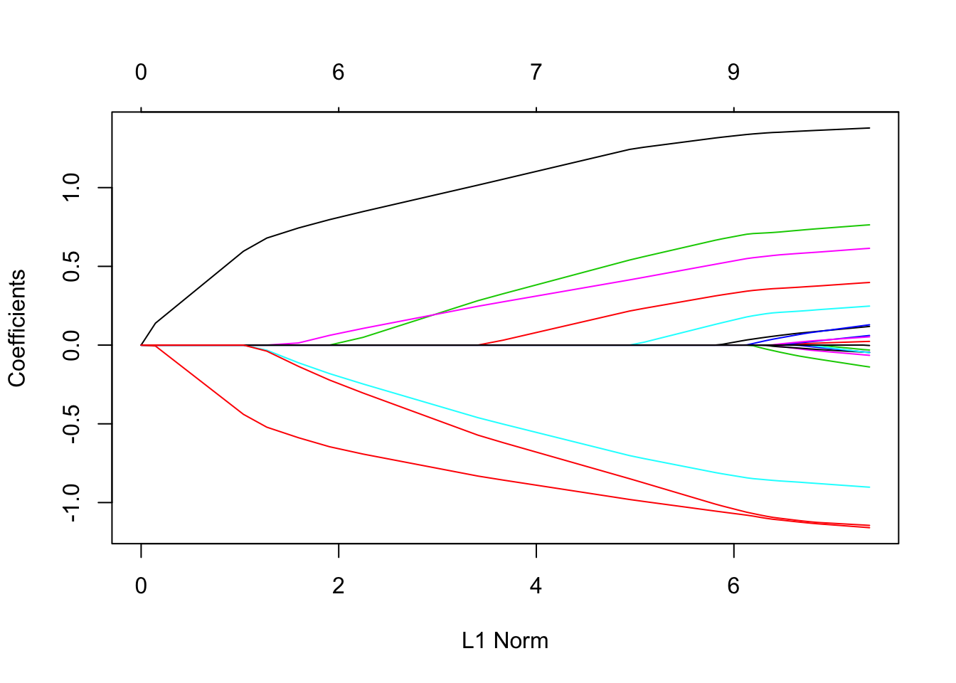
# Simulate a binary response dataset
library(caret)
set.seed(1)
df <- caret::twoClassSim(
  n = 100000,
  linearVars = 10,
  noiseVars = 50,
  corrVars = 50
  )

dim(df)
## [1] 100000    116
# Identify the response & predictor columns
ycol <- "Class"
xcols <- setdiff(names(df), ycol)
df[,ycol] <- ifelse(df[,ycol]=="Class1", 0, 1)
# Split the data into a 70/25% train/test sets
set.seed(1)
idxs <- caret::createDataPartition(y = df[,ycol], p = 0.75)[[1]]
train <- df[idxs,]
test <- df[-idxs,]
train_y <- df[idxs, ycol]
test_y <- df[-idxs, ycol]
train_x <- model.matrix(~-1 + ., train[, xcols])
test_x <- model.matrix(~-1 + ., test[, xcols])
# Dimensions
dim(train_x)
## [1] 75000 115
length(train_y)
## [1] 75000
dim(test_x)
## [1] 25000 115
length(test_y)
## [1] 25000head(test_y)
## [1] 0 1 1 0 0 0# Train a Lasso GLM
system.time(
cvfit <- cv.glmnet(
x = train_x,
y = train_y,
family = "binomial",
alpha = 1.0 # alpha = 1 means lasso by default
)
)
## user system elapsed
## 56.088 1.165 57.369preds <- predict(
cvfit$glmnet.fit,
newx = test_x,
s = cvfit$lambda.min,
type = "response"
)
head(preds)
## 1
## 2 0.3136236
## 14 0.6544411
## 15 0.9269314
## 21 0.1027764
## 29 0.6640567
## 30 0.5079524#install.packages("cvAUC")
library(cvAUC)
cvAUC::AUC(predictions = preds, labels = test_y)
## [1] 0.90828884.7.2 h2o
Introduced in the previous section, the h2o package can perform unregularized or regularized regression. By default, h2o.glm will perform an Elastic Net regression. Similar to the glmnet function, you can adjust the Elastic Net penalty through the alpha parameter (alpha = 1.0 is Lasso and alpha = 0.0 is Ridge).
# Simulate a binary response dataset
library(caret)
set.seed(1)
df <- caret::twoClassSim(
  n = 100000,
  linearVars = 10,
  noiseVars = 50,
  corrVars = 50
  )

dim(df)
## [1] 100000    116
# Convert the data into an H2OFrame
library(h2o)
# initialize h2o instance
h2o.init(nthreads = -1)
##
## H2O is not running yet, starting it now...
##
## Note: In case of errors look at the following log files:
## /var/folders/ws/qs4y2bnx1xs_4y9t0zbdjsvh0000gn/T//Rtmpdbn9Q6/h2o_bradboehmke_started_from_r.out
## /var/folders/ws/qs4y2bnx1xs_4y9t0zbdjsvh0000gn/T//Rtmpdbn9Q6/h2o_bradboehmke_started_from_r.err
##
##
## Starting H2O JVM and connecting: ... Connection successful!
##
## R is connected to the H2O cluster:
## H2O cluster uptime: 2 seconds 823 milliseconds
## H2O cluster timezone: America/New_York
## H2O data parsing timezone: UTC
## H2O cluster version: 3.18.0.4
## H2O cluster version age: 28 days, 3 hours and 12 minutes
## H2O cluster name: H2O_started_from_R_bradboehmke_qca880
## H2O cluster total nodes: 1
## H2O cluster total memory: 1.78 GB
## H2O cluster total cores: 4
## H2O cluster allowed cores: 4
## H2O cluster healthy: TRUE
## H2O Connection ip: localhost
## H2O Connection port: 54321
## H2O Connection proxy: NA
## H2O Internal Security: FALSE
## H2O API Extensions: XGBoost, Algos, AutoML, Core V3, Core V4
## R Version: R version 3.4.4 (2018-03-15)
# Convert the data into an H2OFrame
hf <- as.h2o(df)
##
|
| | 0%
|
|=================================================================| 100%# Identify the response & predictor columns
ycol <- "Class"
xcols <- setdiff(names(hf), ycol)
# Convert the 0/1 binary response to a factor
hf[,ycol] <- as.factor(hf[,ycol])dim(hf)
## [1] 100000 116# Split the data into a 70/25% train/test sets
set.seed(1)
idxs <- caret::createDataPartition(y = df[,ycol], p = 0.75)[[1]]
train <- hf[idxs,]
test <- hf[-idxs,]
# Dimensions
dim(train)
## [1] 75001 116
dim(test)
## [1] 24999 116# Train a Lasso GLM
system.time(
fit <- h2o.glm(
x = xcols,
y = ycol,
training_frame = train,
family = "binomial",
lambda_search = TRUE, # compute lasso path
alpha = 1 # alpha = 1 means lasso, same as glmnet above
)
)
##
|
| | 0%
|
|=== | 4%
|
|============= | 20%
|
|======================= | 36%
|
|================================ | 49%
|
|=================================== | 54%
|
|====================================== | 58%
|
|======================================== | 61%
|
|=================================================================| 100%
## user system elapsed
## 0.449 0.013 8.846# Compute AUC on test dataset
# H2O computes many model performance metrics automatically, including AUC
perf <- h2o.performance(
model = fit,
newdata = test
)
h2o.auc(perf)
## [1] 0.911921# good practice
h2o.shutdown(prompt = FALSE)
## [1] TRUE4.8 References
[1] [https://en.wikipedia.org/wiki/Linear_regression#Generalized\_linear\_models](https://en.wikipedia.org/wiki/Linear_regression#Generalized_linear_models)
[2] [https://en.wikipedia.org/wiki/Generalized\_linear\_model](https://en.wikipedia.org/wiki/Generalized_linear_model)
[3] [Tibshirani, R. (1996). Regression shrinkage and selection via the lasso. J.Royal. Statist. Soc B., Vol. 58, No. 1, pages 267-288).](http://www-stat.stanford.edu/%7Etibs/lasso/lasso.pdf)